Integrating New Report Plugins

The user can define her own report plugins as follows. The default report plugin can be used as a starting point. Entering the name of the default report plugin at R's command line will display the R source code. So,

> spotReportDefault

produces the following output.

spotReportDefault <- function(spotConfig) {		
	spotWriteLines(spotConfig,2,"  Entering spotReportDefault");	
	rawB <- spotGetRawDataMatrixB(spotConfig);
	print(summary(rawB));
	mergedData <- spotPrepareData(spotConfig)
	mergedB <- spotGetMergedDataMatrixB(mergedData, spotConfig);	
	C1 = spotWriteBest(mergedData, spotConfig);
	C1 = C1[C1$COUNT==max(C1$COUNT),];    # choose only among the solutions with high repeat
	cat(sprintf("\n Best solution found with %d evaluations:\n",nrow(rawB)));
	print(C1[1,]);
	fit.tree <- rpart(y ~ ., data= rawB)	
	if (!is.null(fit.tree$splits)){
		if(spotConfig$report.io.pdf==TRUE){ #if pdf should be created
			pdf(spotConfig$io.pdfFileName) #start pdf creation
			spotPlotBst(spotConfig)
			par(mfrow=c(1,1))
			draw.tree(fit.tree, digits=4)	
			dev.off() #close pdf device
		}
		if(spotConfig$report.io.screen==TRUE) #if graphic should be on screen
		{
			x11()
			par(mfrow=c(1,1), xpd=NA)
			draw.tree(fit.tree, digits=4)	
		}
	}	
}

This output can be copied and pasted into a new R file. First, we choose a new name for this plugin, say myReport. This file has to be saved as myReport.R. We choose the actual working directory, i.e., where the java0.* project files reside and where R is started, to save this file. SPOT's function spotGetRawDataMatrixB is used to read the data from the RES file.

myReport <- function(spotConfig) {		
	rawB <- spotGetRawDataMatrixB(spotConfig);		
	...
}

Assuming the user wants to fit a linear regression model to the data, she has to modify the report plugin as follows. In addition to the standard plot of the linear model, she adds a plot of the effects. This plot requires R functions from the effects package, which is loaded via library effects.

myReport <- function(spotConfig) {		
	rawB <- spotGetRawDataMatrixB(spotConfig);
	my.lm <- lm(y ~ ., data= rawB)
	print(summary(my.lm))
	par(mfrow=c(2,2))
	plot(my.lm)	
	library(effects)
	x11()
	plot(allEffects(my.lm), ask=FALSE)
}

Since the new report plugin is located in the actual working directory, the user has to add the line report.path = "." to the CONF file java0.conf. The corresponding lines in the java0.conf has to be modified as follows:

report.func = "myReport"
report.path = "."

That's all. For your convenience, the plugin myReport.R can be downloaded from the workshop's web site.

Executing the command

> spot("java0.conf", rep)

produces the following output.

Call:
lm(formula = y ~ ., data = rawB)

Residuals:
     Min       1Q   Median       3Q      Max 
-0.55087 -0.11698 -0.04086  0.07470  1.11687 

Coefficients:
              Estimate Std. Error t value Pr(>|t|)    
(Intercept) -0.7773069  0.1107214  -7.020 7.20e-12 ***
SIGMANULL    0.0668264  0.0154612   4.322 1.86e-05 ***
VARA         0.8809139  0.1009097   8.730  < 2e-16 ***
VARG         0.0001705  0.0003798   0.449    0.654    
---
Residual standard error: 0.1982 on 503 degrees of freedom
Multiple R-squared: 0.2538,     Adjusted R-squared: 0.2493 
F-statistic: 57.02 on 3 and 503 DF,  p-value: < 2.2e-16

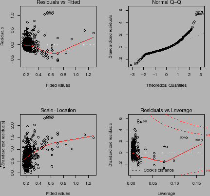
Fig. 5 shows the output from the generic diagnostic plot on the linear model.

Figure 5: Diagnostic plot from the report task 

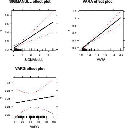
Fig. 6 shows effect plots related to this linear model.

Figure 6: Effect plots from the report task myReport 

Note, since the new report plugin is an R function, it has to be removed from R's workspace, if modifications to the report plugin should have an effect. This can be accomplished by R's rm() command. So, the following commands have to be executed if the report plugin myReport.R is modified several times.

> rm(myReport)
> spot("java0.conf", rep)